Simulate spatial transcriptomic data
Dongyuan Song
Bioinformatics IDP, University of California, Los Angelesdongyuansong@ucla.edu
Qingyang Wang
Department of Statistics, University of California, Los Angelesqw802@g.ucla.edu
15 September 2023
Source:../../scDesign3/code/vignettes/scDesign3-spatial-vignette.Rmd
scDesign3-spatial-vignette.Rmd
library(scDesign3)
library(SingleCellExperiment)
library(ggplot2)
library(dplyr)
library(viridis)
theme_set(theme_bw())
Introduction
In this tutorial, we show how to use scDesign3 to simulate the single-cell spatial data.
Read in the reference data
The raw data is from the Seurat, which is a dataset generated with the Visium technology from 10x Genomics. We pre-select the top spatial variable genes.
example_sce <- readRDS((url("https://figshare.com/ndownloader/files/40582019")))
print(example_sce)
#> class: SingleCellExperiment
#> dim: 1000 2696
#> metadata(0):
#> assays(2): counts logcounts
#> rownames(1000): Calb2 Gng4 ... Fndc5 Gda
#> rowData names(0):
#> colnames(2696): AAACAAGTATCTCCCA-1 AAACACCAATAACTGC-1 ...
#>   TTGTTTCACATCCAGG-1 TTGTTTCCATACAACT-1
#> colData names(12): orig.ident nCount_Spatial ... spatial2 cell_type
#> reducedDimNames(0):
#> mainExpName: NULL
#> altExpNames(0):
To save time, we subset the top 10 genes.
example_sce <- example_sce[1:10, ]Simulation
Then, we can use this spatial dataset to generate new data by setting the parameter mu_formula as a smooth terms for the spatial coordinates.
set.seed(123)
example_simu <- scdesign3(
    sce = example_sce,
    assay_use = "counts",
    celltype = "cell_type",
    pseudotime = NULL,
    spatial = c("spatial1", "spatial2"),
    other_covariates = NULL,
    mu_formula = "s(spatial1, spatial2, bs = 'gp', k= 400)",
    sigma_formula = "1",
    family_use = "nb",
    n_cores = 2,
    usebam = FALSE,
    corr_formula = "1",
    copula = "gaussian",
    DT = TRUE,
    pseudo_obs = FALSE,
    return_model = FALSE,
    nonzerovar = FALSE,
    parallelization = "pbmcapply"
  )
Then, we can create the SinglecellExperiment object using the synthetic count matrix and store the logcounts to the input and synthetic SinglecellExperiment objects.
simu_sce <- SingleCellExperiment(list(counts = example_simu$new_count), colData = example_simu$new_covariate)
logcounts(simu_sce) <- log1p(counts(simu_sce))
Visualization
We reformat the reference data and the synthetic data to visualize a few genes’ expressions and the spatial locations.
VISIUM_dat_test <- data.frame(t(log1p(counts(example_sce)))) %>% as_tibble() %>% dplyr::mutate(X = colData(example_sce)$spatial1, Y = colData(example_sce)$spatial2) %>% tidyr::pivot_longer(-c("X", "Y"), names_to = "Gene", values_to = "Expression") %>% dplyr::mutate(Method = "Reference")
VISIUM_dat_scDesign3 <- data.frame(t(log1p(counts(simu_sce)))) %>% as_tibble() %>% dplyr::mutate(X = colData(simu_sce)$spatial1, Y = colData(simu_sce)$spatial2) %>% tidyr::pivot_longer(-c("X", "Y"), names_to = "Gene", values_to = "Expression") %>% dplyr::mutate(Method = "scDesign3")
VISIUM_dat <- bind_rows(VISIUM_dat_test, VISIUM_dat_scDesign3) %>% dplyr::mutate(Method = factor(Method, levels = c("Reference", "scDesign3")))

VISIUM_dat %>% filter(Gene %in% rownames(example_sce)[1:5]) %>% ggplot(aes(x = X, y = Y, color = Expression)) + geom_point(size = 0.5) + scale_colour_gradientn(colors = viridis_pal(option = "magma")(10), limits=c(0, 8)) + coord_fixed(ratio = 1) + facet_grid(Method ~ Gene )+ theme_gray()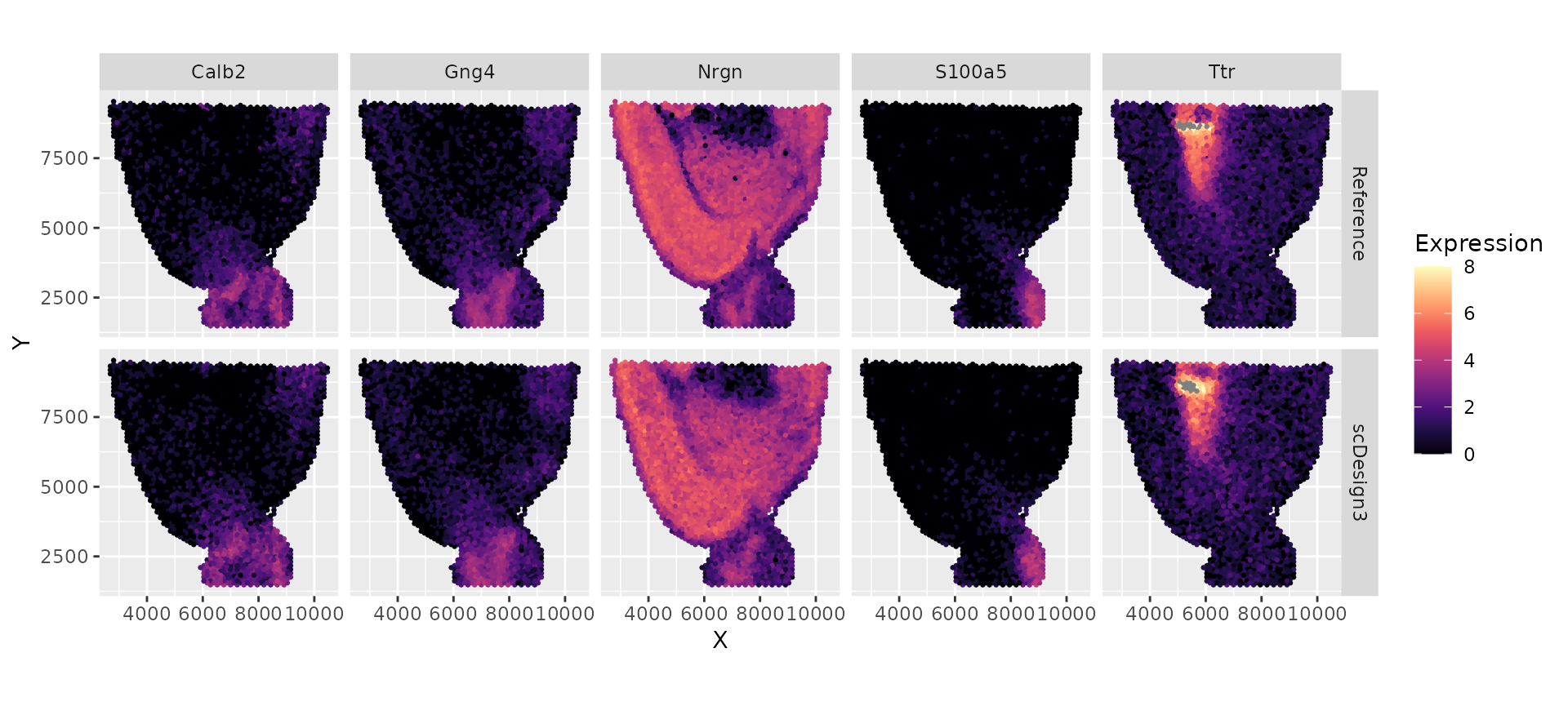
Session information
sessionInfo()
#> R version 4.3.1 (2023-06-16)
#> Platform: x86_64-pc-linux-gnu (64-bit)
#> Running under: Ubuntu 20.04.6 LTS
#>
#> Matrix products: default
#> BLAS:   /usr/lib/x86_64-linux-gnu/openblas-pthread/libblas.so.3
#> LAPACK: /usr/lib/x86_64-linux-gnu/openblas-pthread/liblapack.so.3;  LAPACK version 3.9.0
#>
#> locale:
#>  [1] LC_CTYPE=en_US.UTF-8       LC_NUMERIC=C
#>  [3] LC_TIME=en_US.UTF-8        LC_COLLATE=en_US.UTF-8
#>  [5] LC_MONETARY=en_US.UTF-8    LC_MESSAGES=en_US.UTF-8
#>  [7] LC_PAPER=en_US.UTF-8       LC_NAME=C
#>  [9] LC_ADDRESS=C               LC_TELEPHONE=C
#> [11] LC_MEASUREMENT=en_US.UTF-8 LC_IDENTIFICATION=C
#>
#> time zone: America/Los_Angeles
#> tzcode source: system (glibc)
#>
#> attached base packages:
#> [1] stats4    stats     graphics  grDevices utils     datasets  methods
#> [8] base
#>
#> other attached packages:
#>  [1] viridis_0.6.4               viridisLite_0.4.2
#>  [3] dplyr_1.1.2                 ggplot2_3.4.2
#>  [5] SingleCellExperiment_1.22.0 SummarizedExperiment_1.30.2
#>  [7] Biobase_2.60.0              GenomicRanges_1.52.0
#>  [9] GenomeInfoDb_1.36.1         IRanges_2.34.1
#> [11] S4Vectors_0.38.1            BiocGenerics_0.46.0
#> [13] MatrixGenerics_1.12.2       matrixStats_1.0.0
#> [15] scDesign3_0.99.6            BiocStyle_2.28.0
#>
#> loaded via a namespace (and not attached):
#>  [1] gtable_0.3.3            xfun_0.39               bslib_0.5.0
#>  [4] lattice_0.21-8          gamlss_5.4-12           vctrs_0.6.3
#>  [7] tools_4.3.1             bitops_1.0-7            generics_0.1.3
#> [10] parallel_4.3.1          tibble_3.2.1            fansi_1.0.4
#> [13] highr_0.10              pkgconfig_2.0.3         Matrix_1.6-0
#> [16] desc_1.4.2              lifecycle_1.0.3         GenomeInfoDbData_1.2.10
#> [19] farver_2.1.1            compiler_4.3.1          stringr_1.5.0
#> [22] textshaping_0.3.6       munsell_0.5.0           htmltools_0.5.5
#> [25] sass_0.4.7              RCurl_1.98-1.12         yaml_2.3.7
#> [28] tidyr_1.3.0             crayon_1.5.2            pillar_1.9.0
#> [31] pkgdown_2.0.7           jquerylib_0.1.4         MASS_7.3-60
#> [34] DelayedArray_0.26.6     cachem_1.0.8            mclust_6.0.0
#> [37] nlme_3.1-162            tidyselect_1.2.0        digest_0.6.33
#> [40] mvtnorm_1.2-2           stringi_1.7.12          purrr_1.0.1
#> [43] bookdown_0.34           labeling_0.4.2          splines_4.3.1
#> [46] gamlss.dist_6.0-5       rprojroot_2.0.3         fastmap_1.1.1
#> [49] grid_4.3.1              gamlss.data_6.0-2       colorspace_2.1-0
#> [52] cli_3.6.1               magrittr_2.0.3          S4Arrays_1.0.4
#> [55] survival_3.5-5          utf8_1.2.3              withr_2.5.0
#> [58] scales_1.2.1            XVector_0.40.0          rmarkdown_2.23
#> [61] gridExtra_2.3           ragg_1.2.5              memoise_2.0.1
#> [64] evaluate_0.21           knitr_1.43              mgcv_1.9-0
#> [67] rlang_1.1.1             glue_1.6.2              BiocManager_1.30.21.1
#> [70] jsonlite_1.8.7          R6_2.5.1                zlibbioc_1.46.0
#> [73] systemfonts_1.0.4       fs_1.6.3