Evaluate pseudotime goodness-of-fit by scDesign3
Dongyuan Song
Bioinformatics IDP, University of California, Los Angelesdongyuansong@ucla.edu
Qingyang Wang
Department of Statistics, University of California, Los Angelesqw802@g.ucla.edu
15 September 2023
Source:../../scDesign3/code/vignettes/scDesign3-pseudotimeGOF-vignette.Rmd
scDesign3-pseudotimeGOF-vignette.Rmd
library(scDesign3)
library(dyngen)
library(SingleCellExperiment)
library(ggplot2)
library(dplyr)
theme_set(theme_bw())
Introduction
In this tutorial, we will show how to use scDesign3 to evaluate the pseudotime goodness-of-fit for different pseudotime labels. If the true labels are unavailable and we have little prior knowledge, the scDesign3 BIC can serve as an unsupervised metric. In this tutorial, we will first use the R package dyngen to generate a dataset with ground truth "pseudotime". Then, we will perturb the ground truth pseudotime to worsen its quality and use scDesign3’s BIC to examine pseudotime goodness-of-fit.
Generation of reference dataset & Simulation
We will first use dyngen to generate a dataset with ground truth “pseudotime”.
set.seed(123)
backbone <- backbone_linear_simple()
config <-
  initialise_model(
    backbone = backbone,
    num_cells = 500,
    num_tfs = nrow(backbone$module_info),
    num_targets = 100,
    num_hks = 50,
    verbose = FALSE
  )
out <- generate_dataset(
  config,
  format = "sce",
  make_plots = FALSE
  )
example_sce <- out$dataset
colData(example_sce)$pseudotime <- out$model$experiment$cell_info$time
Secondly, we perturb the pseudotime by generating random numbers from uniform distribution and replacing various percentages of the original pseudotime with random numbers. The percentage ranges from 0% to 100%. In the code below, we generate 11 sets of perturbed pseudotime with the percentage of perturbation ranging from 0% to 100%. For each new set of perturbed pseudotime, we create a new SingleCellExperiment object, storing the original count matrix and the corresponding perturbed pseudotime.
set.seed(123)
example_sce_list <- lapply(0:10, function(x) {
  perturb_prop <- x/10
  n_cell <- round(dim(example_sce)[2]*perturb_prop)
  cell_index <- sample(1:dim(example_sce)[2], n_cell)

  new_pseudotime <- colData(example_sce)$pseudotime
  new_pseudotime[cell_index] <- runif(n_cell)

  curr_sce <- example_sce
  colData(curr_sce)$pseudotime <- new_pseudotime
  curr_sce
})
Thirdly, we iteratively run the function scdesign3; each iteration uses a different set of pseudotime that we generated above.
set.seed(123)
scDesign3_result <- lapply(example_sce_list, function(x) {
  res <-  scdesign3(
    sce = x,
    assay_use = "counts",
    celltype = NULL,
    pseudotime = "pseudotime",
    spatial = NULL,
    other_covariates = NULL,
    mu_formula = "s(pseudotime, bs = 'cr', k = 10)",
    sigma_formula = "1",
    corr_formula = "ind",
    copula = "gaussian",
    n_cores = 2
  )
  return(res)
})
Visualization
After the simulations, we first extract out scDesign3’s BIC, which is an unsupervised metric for evaluating the goodness-of-fit of the pseudotime.
bic_list <- lapply(scDesign3_result, function(x){return(x$model_bic)})
bic_df <- data.frame(matrix(unlist(bic_list), nrow = length(bic_list), byrow = TRUE))
colnames(bic_df) <- names(bic_list[[1]])
bic_df
#>    bic.marginal bic.copula bic.total
#> 1      463280.2          0  463280.2
#> 2      499829.7          0  499829.7
#> 3      512349.0          0  512349.0
#> 4      516330.9          0  516330.9
#> 5      522417.5          0  522417.5
#> 6      525315.8          0  525315.8
#> 7      528644.0          0  528644.0
#> 8      532390.2          0  532390.2
#> 9      533014.4          0  533014.4
#> 10     534671.6          0  534671.6
#> 11     533596.2          0  533596.2
Since we also have the ground truth pseudotime, we also calculate the \(r^2\) between the ground truth pseudotime and perturbed pseudotime. The \(r^2\) is a supervised metric to evaluate the pseudotime qualities. The figure below demonstrates that scDesign3’s BIC agrees with \(r^2\).
r2 <- sapply(example_sce_list, function(x){
  cor(colData(example_sce_list[[1]])$pseudotime, colData(x)$pseudotime)^2
})
metric <- tibble(bic = bic_df$bic.marginal, r2 = r2, Method = paste0("perturb ",seq(0,100,by = 10), "%"))
p_pseudotime_metric <- metric %>% ggplot(aes(x = r2, y = bic,label = Method)) + geom_point() + theme_bw() + theme(aspect.ratio = 1,
    panel.grid.minor = element_blank(),
    panel.grid.major = element_blank()) + ggpubr::stat_cor(method = "spearman", cor.coef.name = "rho", label.x.npc = "left", label.y.npc = 0.5) + ylab("scDesign3 BIC") + xlab("R2 (truth vs pseudotime)")
p_pseudotime_metric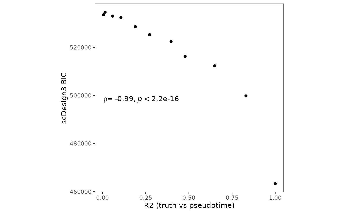
Session information
sessionInfo()
#> R version 4.3.1 (2023-06-16)
#> Platform: x86_64-pc-linux-gnu (64-bit)
#> Running under: Ubuntu 20.04.6 LTS
#>
#> Matrix products: default
#> BLAS:   /usr/lib/x86_64-linux-gnu/openblas-pthread/libblas.so.3
#> LAPACK: /usr/lib/x86_64-linux-gnu/openblas-pthread/liblapack.so.3;  LAPACK version 3.9.0
#>
#> locale:
#>  [1] LC_CTYPE=en_US.UTF-8       LC_NUMERIC=C
#>  [3] LC_TIME=en_US.UTF-8        LC_COLLATE=en_US.UTF-8
#>  [5] LC_MONETARY=en_US.UTF-8    LC_MESSAGES=en_US.UTF-8
#>  [7] LC_PAPER=en_US.UTF-8       LC_NAME=C
#>  [9] LC_ADDRESS=C               LC_TELEPHONE=C
#> [11] LC_MEASUREMENT=en_US.UTF-8 LC_IDENTIFICATION=C
#>
#> time zone: America/Los_Angeles
#> tzcode source: system (glibc)
#>
#> attached base packages:
#> [1] stats4    stats     graphics  grDevices utils     datasets  methods
#> [8] base
#>
#> other attached packages:
#>  [1] dplyr_1.1.2                 ggplot2_3.4.2
#>  [3] SingleCellExperiment_1.22.0 SummarizedExperiment_1.30.2
#>  [5] Biobase_2.60.0              GenomicRanges_1.52.0
#>  [7] GenomeInfoDb_1.36.1         IRanges_2.34.1
#>  [9] S4Vectors_0.38.1            BiocGenerics_0.46.0
#> [11] MatrixGenerics_1.12.2       matrixStats_1.0.0
#> [13] dyngen_1.0.5                scDesign3_0.99.6
#> [15] BiocStyle_2.28.0
#>
#> loaded via a namespace (and not attached):
#>   [1] bitops_1.0-7            pbapply_1.7-2           gridExtra_2.3
#>   [4] remotes_2.4.2.1         rlang_1.1.1             magrittr_2.0.3
#>   [7] gamlss_5.4-12           compiler_4.3.1          mgcv_1.9-0
#>  [10] systemfonts_1.0.4       vctrs_0.6.3             stringr_1.5.0
#>  [13] pkgconfig_2.0.3         crayon_1.5.2            fastmap_1.1.1
#>  [16] backports_1.4.1         XVector_0.40.0          labeling_0.4.2
#>  [19] lmds_0.1.0              ggraph_2.1.0            utf8_1.2.3
#>  [22] rmarkdown_2.23          tzdb_0.4.0              ragg_1.2.5
#>  [25] purrr_1.0.1             xfun_0.39               zlibbioc_1.46.0
#>  [28] cachem_1.0.8            jsonlite_1.8.7          highr_0.10
#>  [31] DelayedArray_0.26.6     tweenr_2.0.2            broom_1.0.5
#>  [34] irlba_2.3.5.1           parallel_4.3.1          R6_2.5.1
#>  [37] bslib_0.5.0             stringi_1.7.12          car_3.1-2
#>  [40] jquerylib_0.1.4         Rcpp_1.0.11             bookdown_0.34
#>  [43] assertthat_0.2.1        knitr_1.43              readr_2.1.4
#>  [46] dynutils_1.0.11         Matrix_1.6-0            splines_4.3.1
#>  [49] igraph_1.5.0.1          tidyselect_1.2.0        abind_1.4-5
#>  [52] yaml_2.3.7              viridis_0.6.4           gamlss.dist_6.0-5
#>  [55] codetools_0.2-19        lattice_0.21-8          tibble_3.2.1
#>  [58] withr_2.5.0             evaluate_0.21           desc_1.4.2
#>  [61] survival_3.5-5          RcppParallel_5.1.7      polyclip_1.10-4
#>  [64] mclust_6.0.0            ggpubr_0.6.0            pillar_1.9.0
#>  [67] BiocManager_1.30.21.1   carData_3.0-5           generics_0.1.3
#>  [70] rprojroot_2.0.3         RCurl_1.98-1.12         hms_1.1.3
#>  [73] munsell_0.5.0           scales_1.2.1            RcppXPtrUtils_0.1.2
#>  [76] glue_1.6.2              proxyC_0.3.3            tools_4.3.1
#>  [79] ggsignif_0.6.4          fs_1.6.3                graphlayouts_1.0.0
#>  [82] tidygraph_1.2.3         GillespieSSA2_0.3.0     grid_4.3.1
#>  [85] tidyr_1.3.0             colorspace_2.1-0        nlme_3.1-162
#>  [88] GenomeInfoDbData_1.2.10 patchwork_1.1.2         ggforce_0.4.1
#>  [91] cli_3.6.1               textshaping_0.3.6       fansi_1.0.4
#>  [94] S4Arrays_1.0.4          viridisLite_0.4.2       gtable_0.3.3
#>  [97] rstatix_0.7.2           sass_0.4.7              digest_0.6.33
#> [100] gamlss.data_6.0-2       ggrepel_0.9.3           farver_2.1.1
#> [103] memoise_2.0.1           htmltools_0.5.5         pkgdown_2.0.7
#> [106] lifecycle_1.0.3         MASS_7.3-60