Simulate datasets with condition effect
Dongyuan Song
Bioinformatics IDP, University of California, Los Angelesdongyuansong@ucla.edu
Qingyang Wang
Department of Statistics, University of California, Los Angelesqw802@g.ucla.edu
15 September 2023
Source:../../scDesign3/code/vignettes/scDesign3-conditionEffect-vignette.Rmd
scDesign3-conditionEffect-vignette.RmdIntroduction
In this tutorial, we will show how to use scDesign3 to simulate data with condition effects and how to adjust the condition effects.
Read in the reference data
The raw data is from the SeuratData package. The data is called ifnb in the package; it is PBMC data simulated and controlled by IFNB.
example_sce <- readRDS((url("https://figshare.com/ndownloader/files/40581977")))
print(example_sce)
#> class: SingleCellExperiment
#> dim: 1000 13999
#> metadata(0):
#> assays(2): counts logcounts
#> rownames(1000): FTL HBB ... AC022182.3 SCIN
#> rowData names(0):
#> colnames(13999): AAACATACATTTCC.1 AAACATACCAGAAA.1 ... TTTGCATGCTAAGC.1
#>   TTTGCATGGGACGA.1
#> colData names(8): orig.ident nCount_RNA ... cell_type condition
#> reducedDimNames(0):
#> mainExpName: RNA
#> altExpNames(0):
print(table(colData(example_sce)$cell_type))
#>
#>    CD14 Mono  CD4 Naive T CD4 Memory T    CD16 Mono            B        CD8 T
#>         4362         2504         1762         1044          978          814
#>  T activated           NK           DC  B Activated           Mk          pDC
#>          633          619          472          388          236          132
#>        Eryth
#>           55
To save computational time, we only use the top 100 genes and two cell types (CD14 Mono and B).
example_sce <- example_sce[1:100, colData(example_sce)$cell_type %in% c("CD14 Mono", "B")]

## Remove unused cell type levels
colData(example_sce)$cell_type <- droplevels(colData(example_sce)$cell_type)
The condition information is stored in colData of the example dataset.
head(colData(example_sce))
#> DataFrame with 6 rows and 8 columns
#>                   orig.ident nCount_RNA nFeature_RNA        stim
#>                  <character>  <numeric>    <integer> <character>
#> AAACATACATTTCC.1 IMMUNE_CTRL       3017          877        CTRL
#> AAACATACCAGAAA.1 IMMUNE_CTRL       2481          713        CTRL
#> AAACATACCTCGCT.1 IMMUNE_CTRL       3420          850        CTRL
#> AAACATACGGCATT.1 IMMUNE_CTRL       1581          557        CTRL
#> AAACATTGCTTCGC.1 IMMUNE_CTRL       2536          669        CTRL
#> AAACGCACTCGCCT.1 IMMUNE_CTRL       3563          908        CTRL
#>                  seurat_annotations       ident cell_type   condition
#>                            <factor>    <factor>  <factor> <character>
#> AAACATACATTTCC.1          CD14 Mono IMMUNE_CTRL CD14 Mono        CTRL
#> AAACATACCAGAAA.1          CD14 Mono IMMUNE_CTRL CD14 Mono        CTRL
#> AAACATACCTCGCT.1          CD14 Mono IMMUNE_CTRL CD14 Mono        CTRL
#> AAACATACGGCATT.1          CD14 Mono IMMUNE_CTRL CD14 Mono        CTRL
#> AAACATTGCTTCGC.1          CD14 Mono IMMUNE_CTRL CD14 Mono        CTRL
#> AAACGCACTCGCCT.1          CD14 Mono IMMUNE_CTRL CD14 Mono        CTRL
Simulation
First, we will simulate new data with the condition effects.
set.seed(123)
simu_res <- scdesign3(
    sce = example_sce,
    assay_use = "counts",
    celltype = "cell_type",
    pseudotime = NULL,
    spatial = NULL,
    other_covariates = c("condition"),
    mu_formula = "cell_type + condition + cell_type*condition",
    sigma_formula = "1",
    family_use = "nb",
    n_cores = 2,
    usebam = FALSE,
    corr_formula = "cell_type",
    copula = "gaussian",
    DT = TRUE,
    pseudo_obs = FALSE,
    return_model = FALSE,
    nonzerovar = FALSE
  )
Then, we can also simulate a new dataset with condition effects on B cells removed.
IFNB_data <- construct_data(
  sce = example_sce,
  assay_use = "counts",
  celltype = "cell_type",
  pseudotime = NULL,
  spatial = NULL,
  other_covariates = c("condition"),
  corr_by = "cell_type"
)
IFNB_marginal <- fit_marginal(
  data = IFNB_data,
  predictor = "gene",
  mu_formula = "cell_type + condition + cell_type*condition",
  sigma_formula = "1",
  family_use = "nb",
  n_cores = 2,
  usebam = FALSE
)
set.seed(123)
IFNB_copula <- fit_copula(
    sce = example_sce,
    assay_use = "counts",
    marginal_list = IFNB_marginal,
    family_use = "nb",
    copula = "gaussian",
    n_cores = 2,
    input_data = IFNB_data$dat
  )
In here, the condition effects on B cells are removed for all genes by modifying the estimated coefficients for all genes’ marginal models.
IFNB_marginal_null_B <- lapply(IFNB_marginal, function(x) {
  x$fit$coefficients["cell_typeB:conditionSTIM"] <- 0-x$fit$coefficients["conditionSTIM"]
  x
})
Then, we can generate the parameters using the altered marginal fits and simulate new data with the altered paremeters.
IFNB_para_null_B <- extract_para(
    sce = example_sce,
    marginal_list = IFNB_marginal_null_B,
    n_cores = 2,
    family_use = "nb",
    new_covariate = IFNB_data$newCovariate,
    data = IFNB_data$dat
  )
set.seed(123)
IFNB_newcount_null_B <- simu_new(
    sce = example_sce,
    mean_mat = IFNB_para_null_B$mean_mat,
    sigma_mat = IFNB_para_null_B$sigma_mat,
    zero_mat = IFNB_para_null_B$zero_mat,
    quantile_mat = NULL,
    copula_list = IFNB_copula$copula_list,
    n_cores = 2,
    family_use = "nb",
    input_data = IFNB_data$dat,
    new_covariate = IFNB_data$newCovariate,
    important_feature = IFNB_copula$important_feature,
    filtered_gene = IFNB_data$filtered_gene
  )
Then, we can create the SinglecellExperiment object using the synthetic count matrix and store the logcounts to the input and synthetic SinglecellExperiment objects.
Visulization
set.seed(123)
compare_figure <- plot_reduceddim(ref_sce = example_sce,
                                  sce_list = simu_res_list,
                                  name_vec = c("Reference", "w/ Condition", "Modified Condition"),
                                  assay_use = "logcounts",
                                  if_plot = TRUE,
                                  color_by = "cell_type",
                                  shape_by = "condition",
                                  n_pc = 20)
plot(compare_figure$p_umap)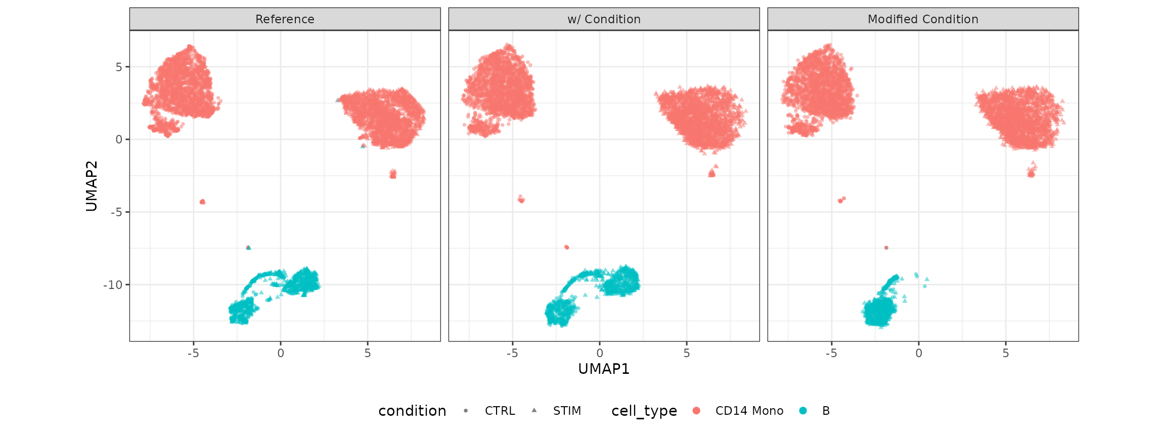
Session information
sessionInfo()
#> R version 4.3.1 (2023-06-16)
#> Platform: x86_64-pc-linux-gnu (64-bit)
#> Running under: Ubuntu 20.04.6 LTS
#>
#> Matrix products: default
#> BLAS:   /usr/lib/x86_64-linux-gnu/openblas-pthread/libblas.so.3
#> LAPACK: /usr/lib/x86_64-linux-gnu/openblas-pthread/liblapack.so.3;  LAPACK version 3.9.0
#>
#> locale:
#>  [1] LC_CTYPE=en_US.UTF-8       LC_NUMERIC=C
#>  [3] LC_TIME=en_US.UTF-8        LC_COLLATE=en_US.UTF-8
#>  [5] LC_MONETARY=en_US.UTF-8    LC_MESSAGES=en_US.UTF-8
#>  [7] LC_PAPER=en_US.UTF-8       LC_NAME=C
#>  [9] LC_ADDRESS=C               LC_TELEPHONE=C
#> [11] LC_MEASUREMENT=en_US.UTF-8 LC_IDENTIFICATION=C
#>
#> time zone: America/Los_Angeles
#> tzcode source: system (glibc)
#>
#> attached base packages:
#> [1] stats4    stats     graphics  grDevices utils     datasets  methods
#> [8] base
#>
#> other attached packages:
#>  [1] ggplot2_3.4.2               SingleCellExperiment_1.22.0
#>  [3] SummarizedExperiment_1.30.2 Biobase_2.60.0
#>  [5] GenomicRanges_1.52.0        GenomeInfoDb_1.36.1
#>  [7] IRanges_2.34.1              S4Vectors_0.38.1
#>  [9] BiocGenerics_0.46.0         MatrixGenerics_1.12.2
#> [11] matrixStats_1.0.0           scDesign3_0.99.6
#> [13] BiocStyle_2.28.0
#>
#> loaded via a namespace (and not attached):
#>  [1] tidyselect_1.2.0        farver_2.1.1            dplyr_1.1.2
#>  [4] bitops_1.0-7            fastmap_1.1.1           RCurl_1.98-1.12
#>  [7] digest_0.6.33           lifecycle_1.0.3         survival_3.5-5
#> [10] gamlss.dist_6.0-5       magrittr_2.0.3          compiler_4.3.1
#> [13] rlang_1.1.1             sass_0.4.7              tools_4.3.1
#> [16] utf8_1.2.3              yaml_2.3.7              knitr_1.43
#> [19] askpass_1.1             S4Arrays_1.0.4          labeling_0.4.2
#> [22] mclust_6.0.0            reticulate_1.30         DelayedArray_0.26.6
#> [25] withr_2.5.0             purrr_1.0.1             desc_1.4.2
#> [28] grid_4.3.1              fansi_1.0.4             colorspace_2.1-0
#> [31] scales_1.2.1            MASS_7.3-60             cli_3.6.1
#> [34] mvtnorm_1.2-2           rmarkdown_2.23          crayon_1.5.2
#> [37] ragg_1.2.5              generics_0.1.3          umap_0.2.10.0
#> [40] RSpectra_0.16-1         cachem_1.0.8            stringr_1.5.0
#> [43] zlibbioc_1.46.0         splines_4.3.1           parallel_4.3.1
#> [46] BiocManager_1.30.21.1   XVector_0.40.0          vctrs_0.6.3
#> [49] Matrix_1.6-0            jsonlite_1.8.7          bookdown_0.34
#> [52] gamlss_5.4-12           irlba_2.3.5.1           systemfonts_1.0.4
#> [55] jquerylib_0.1.4         glue_1.6.2              pkgdown_2.0.7
#> [58] stringi_1.7.12          gtable_0.3.3            munsell_0.5.0
#> [61] tibble_3.2.1            pillar_1.9.0            htmltools_0.5.5
#> [64] openssl_2.1.0           gamlss.data_6.0-2       GenomeInfoDbData_1.2.10
#> [67] R6_2.5.1                textshaping_0.3.6       rprojroot_2.0.3
#> [70] evaluate_0.21           lattice_0.21-8          highr_0.10
#> [73] png_0.1-8               memoise_2.0.1           bslib_0.5.0
#> [76] Rcpp_1.0.11             nlme_3.1-162            mgcv_1.9-0
#> [79] xfun_0.39               fs_1.6.3                pkgconfig_2.0.3