Simulate spot-resolution spatial data for cell-type deconvolution
Dongyuan Song
Bioinformatics IDP, University of California, Los Angelesdongyuansong@ucla.edu
Qingyang Wang
Department of Statistics, University of California, Los Angelesqw802@g.ucla.edu
15 September 2023
Source:../../scDesign3/code/vignettes/scDesign3-spatial-deconvolution.Rmd
scDesign3-spatial-deconvolution.Rmd
library(scDesign3)
library(SingleCellExperiment)
library(ggplot2)
library(dplyr)
library(viridis)
library(IOBR)
library(scatterpie)
theme_set(theme_bw())
Introduction
In this tutorial, we show how to use scDesign3 to simulate the spot-resolution spatial data, which each spot is a mix of cells from different cell types.
Read in the reference data
The paired scRNA-seq and spatial data were used in CARD. We pre-select the top cell-type marker genes.
MOBSC_sce <- readRDS((url("https://figshare.com/ndownloader/files/40581983")))
MOBSP_sce <- readRDS((url("https://figshare.com/ndownloader/files/40581986")))
print(MOBSC_sce)
#> class: SingleCellExperiment
#> dim: 182 12640
#> metadata(0):
#> assays(2): counts logcounts
#> rownames(182): Grin2b Prkca ... Zic1 Tpi1
#> rowData names(1): rownames.count.
#> colnames(12640): WT1_AAACCTGAGCTGCGAA WT1_AAACCTGGTTTGGCGC ...
#>   OC2_TAGTTGGTCGCGATCG OC2_TTGCGTCAGGATCGCA
#> colData names(4): cellType sampleInfo sizeFactor cell_type
#> reducedDimNames(0):
#> mainExpName: NULL
#> altExpNames(0):
print(MOBSP_sce)
#> class: SingleCellExperiment
#> dim: 182 278
#> metadata(0):
#> assays(1): counts
#> rownames(182): Grin2b Prkca ... Zic1 Tpi1
#> rowData names(0):
#> colnames(278): 16.918x16.996 18.017x17.034 ... 25.134x28.934
#>   29.961x18.97
#> colData names(2): spatial1 spatial2
#> reducedDimNames(0):
#> mainExpName: NULL
#> altExpNames(0):Simulation
We first use scDesign3 to estimate the cell-type reference from scRNA-seq data.
set.seed(123)
MOBSC_data <- construct_data(
  sce = MOBSC_sce,
  assay_use = "counts",
  celltype = "cell_type",
  pseudotime = NULL,
  spatial = NULL,
  other_covariates = NULL,
  corr_by = "1"
)

MOBSC_marginal <- fit_marginal(
  data = MOBSC_data,
  predictor = "gene",
  mu_formula = "cell_type",
  sigma_formula = "cell_type",
  family_use = "nb",
  n_cores = 2,
  usebam = FALSE,
  parallelization = "pbmcmapply"

)

MOBSC_copula <- fit_copula(
  sce = MOBSC_sce,
  assay_use = "counts",
  marginal_list = MOBSC_marginal,
  family_use = "nb",
  copula = "gaussian",
  n_cores = 2,
  input_data = MOBSC_data$dat
)

MOBSC_para <- extract_para(
  sce = MOBSC_sce,
  marginal_list = MOBSC_marginal,
  n_cores = 2,
  family_use = "nb",
  new_covariate = MOBSC_data$newCovariate,
  data = MOBSC_data$dat
)

MOBSC_newcount <- simu_new(
  sce = MOBSC_sce,
  mean_mat = MOBSC_para$mean_mat,
  sigma_mat = MOBSC_para$sigma_mat,
  zero_mat = MOBSC_para$zero_mat,
  quantile_mat = NULL,
  copula_list = MOBSC_copula$copula_list,
  n_cores = 2,
  family_use = "nb",
  input_data = MOBSC_data$dat,
  new_covariate = MOBSC_data$newCovariate,
  filtered_gene = MOBSC_data$filtered_gene
)
set.seed(123)
MOBSP_data <- construct_data(
  sce = MOBSP_sce,
  assay_use = "counts",
  celltype = NULL,
  pseudotime = NULL,
  spatial = c("spatial1", "spatial2"),
  other_covariates = NULL,
  corr_by = "1"
)

MOBSP_marginal <- fit_marginal(
  data = MOBSP_data,
  predictor = "gene",
  mu_formula = "s(spatial1, spatial2, bs = 'gp', k = 50, m = c(1, 2, 1))",
  sigma_formula = "1",
  family_use = "nb",
  n_cores = 2,
  usebam = FALSE,
  parallelization = "pbmcmapply"

)

MOBSP_copula <- fit_copula(
  sce = MOBSP_sce,
  assay_use = "counts",
  marginal_list = MOBSP_marginal,
  family_use = "nb",
  copula = "gaussian",
  n_cores = 2,
  input_data = MOBSP_data$dat
)

MOBSP_para <- extract_para(
  sce = MOBSP_sce,
  marginal_list = MOBSP_marginal,
  n_cores = 2,
  family_use = "nb",
  new_covariate = MOBSP_data$newCovariate,
  data = MOBSP_data$dat
)
Now we get the fitted models for scRNA-seq and spatial data. We need to extract their mean parameters (i.e., expected expression values).
MOBSC_sig_matrix <- sapply(cell_type, function(x) {
  rowMeans(t(MOBSC_para$mean_mat)[, colData(MOBSC_sce)$cellType %in% x])
})

MOBSP_matrix <- (t(MOBSP_para$mean_mat))
We use CIBERSORT to decompose each spot’s expected expression into cell-type proportions. This step is to set the true cell-type proportions. Please note you can also use other decomposition methods or set the proportion mannully if you have your own design.
sig_matrix <- as.data.frame(MOBSC_sig_matrix)
mixture_file <- as.data.frame(MOBSP_matrix)

proportion_mat <- IOBR::CIBERSORT(sig_matrix, mixture_file, QN = FALSE, absolute = FALSE, perm = 10)
proportion_mat <- proportion_mat[, 1:4]
We can visualzie the proportions by pie-chart.
colors_cell_type <- c("#E69F00", "#56B4E9", "#009E73",
                       "#0072B2")
d_pie <- as_tibble(colData(MOBSP_sce), rownames = "cell") %>% bind_cols(as_tibble(proportion_mat)) %>% dplyr::mutate(region = seq_len(dim(MOBSP_sce)[2])) %>% dplyr::mutate(X= spatial1, Y = spatial2)

p_pie_plot <- ggplot() + geom_scatterpie(aes(x=X, y=Y, group=region), data=d_pie ,
                           cols = cell_type, color=NA) + coord_fixed(ratio = 1) +
                                scale_fill_manual(values = colors_cell_type) + coord_equal()+ theme_bw() + theme(legend.position = "left")  + theme(
    panel.grid.minor = element_blank(),
    panel.grid.major = element_blank(),
    axis.text.x=element_blank(),
    axis.ticks.x=element_blank(),
    axis.text.y=element_blank(),
    axis.ticks.y=element_blank())+ guides(fill=guide_legend(title="Cell type"))
p_pie_plot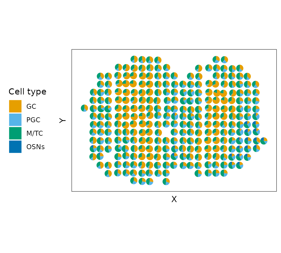
Then we can simulate new spatial data where each spot is the sum of 50 cells/5 (therefore on average 10 cells per spot). Increasing the number of cells will make the spatial data smoother (closer to the expected spatial expression).
set.seed(123)
MOBSCSIM_sce <- MOBSC_sce
counts(MOBSCSIM_sce) <- MOBSC_newcount

MOBSP_new_mixture <- (apply(proportion_mat, 1, function(x) {
  n = 50
  rowSums(sapply(cell_type, function(y) {
    index <- sample(which(colData(MOBSCSIM_sce)$cell_type==y), size = n, replace = FALSE)
    rowSums(MOBSC_newcount[, index])*x[y]
  }))
}))

MOBSP_new_mixture <- MOBSP_new_mixture/5

### Ceiling to integer
MOBSP_new_mixture <- ceiling(MOBSP_new_mixture)

MOBSPMIX_sce <- MOBSP_sce
counts(MOBSPMIX_sce) <- as.matrix(MOBSP_new_mixture)
Finally, we can check the simulated results. We use four cell-type marker genes as the example.
MOBSC_sig_matrix <- sapply(cell_type, function(x) {
  rowMeans(t(MOBSC_para$mean_mat)[, colData(MOBSC_sce)$cellType %in% x])
})
MOBSP_sc_mixture <- tcrossprod(as.matrix(MOBSC_sig_matrix), as.matrix(proportion_mat))

rownames(MOBSP_sc_mixture) <- rownames(MOBSP_new_mixture)

location <- colData(MOBSP_sce)
MOBSP_real_tbl <- as_tibble(t(log1p(counts(MOBSP_sce)))) %>% dplyr::mutate(X = location$spatial1,
                                             Y = location$spatial2) %>%
  tidyr::pivot_longer(-c("X", "Y"), names_to = "Gene", values_to = "Expression") %>% dplyr::mutate(Method = "Real data")

MOBSP_real_tbl <- transform(MOBSP_real_tbl, Expression=ave(Expression, Gene, FUN=scales::rescale))


MOBSP_mixture_tbl <- as_tibble(t(log1p(MOBSP_new_mixture))) %>% dplyr::mutate(X = location$spatial1,
                                             Y = location$spatial2) %>%
  tidyr::pivot_longer(-c("X", "Y"), names_to = "Gene", values_to = "Expression") %>% dplyr::mutate(Method = "scDesign3")

MOBSP_mixture_tbl <- transform(MOBSP_mixture_tbl, Expression=ave(Expression, Gene, FUN=scales::rescale))

MOBSP_tbl <- bind_rows(list(MOBSP_real_tbl, MOBSP_mixture_tbl))

MOBSC_marker <- c("Penk", "Apold1", "Cdhr1", "S100a5")

p_MOB_prop <- MOBSP_tbl %>% dplyr::filter(Gene %in% MOBSC_marker) %>% dplyr::mutate(Gene = factor(Gene, levels = MOBSC_marker)) %>% ggplot(aes(x = X, y = Y, color = Expression))  + ggrastr::rasterize(geom_point(size = 1), dpi = 300) + scale_colour_gradientn(colors = viridis_pal(option = "B", direction = -1)(10), limits=c(0, 1)) + coord_fixed(ratio = 1) + facet_grid(Method ~ Gene ) + theme_bw() + theme(legend.position = "right")  + theme(
    panel.grid.minor = element_blank(),
    panel.grid.major = element_blank(),
    axis.text.x=element_blank(),
    axis.ticks.x=element_blank(),
    axis.text.y=element_blank(),
    axis.ticks.y=element_blank())
p_MOB_prop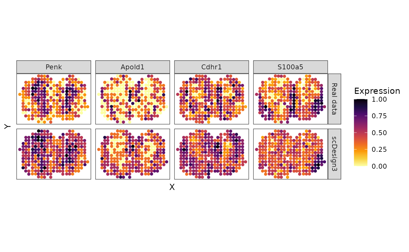
Session information
sessionInfo()
#> R version 4.3.1 (2023-06-16)
#> Platform: x86_64-pc-linux-gnu (64-bit)
#> Running under: Ubuntu 20.04.6 LTS
#>
#> Matrix products: default
#> BLAS:   /usr/lib/x86_64-linux-gnu/openblas-pthread/libblas.so.3
#> LAPACK: /usr/lib/x86_64-linux-gnu/openblas-pthread/liblapack.so.3;  LAPACK version 3.9.0
#>
#> locale:
#>  [1] LC_CTYPE=en_US.UTF-8       LC_NUMERIC=C
#>  [3] LC_TIME=en_US.UTF-8        LC_COLLATE=en_US.UTF-8
#>  [5] LC_MONETARY=en_US.UTF-8    LC_MESSAGES=en_US.UTF-8
#>  [7] LC_PAPER=en_US.UTF-8       LC_NAME=C
#>  [9] LC_ADDRESS=C               LC_TELEPHONE=C
#> [11] LC_MEASUREMENT=en_US.UTF-8 LC_IDENTIFICATION=C
#>
#> time zone: America/Los_Angeles
#> tzcode source: system (glibc)
#>
#> attached base packages:
#> [1] grid      stats4    stats     graphics  grDevices utils     datasets
#> [8] methods   base
#>
#> other attached packages:
#>  [1] scatterpie_0.2.1            IOBR_0.99.9
#>  [3] tidyHeatmap_1.8.1           ComplexHeatmap_2.16.0
#>  [5] survival_3.5-5              ggpubr_0.6.0
#>  [7] tibble_3.2.1                viridis_0.6.4
#>  [9] viridisLite_0.4.2           dplyr_1.1.2
#> [11] ggplot2_3.4.2               SingleCellExperiment_1.22.0
#> [13] SummarizedExperiment_1.30.2 Biobase_2.60.0
#> [15] GenomicRanges_1.52.0        GenomeInfoDb_1.36.1
#> [17] IRanges_2.34.1              S4Vectors_0.38.1
#> [19] BiocGenerics_0.46.0         MatrixGenerics_1.12.2
#> [21] matrixStats_1.0.0           scDesign3_0.99.6
#> [23] BiocStyle_2.28.0
#>
#> loaded via a namespace (and not attached):
#>   [1] splines_4.3.1             bitops_1.0-7
#>   [3] polyclip_1.10-4           preprocessCore_1.62.1
#>   [5] graph_1.78.0              XML_3.99-0.14
#>   [7] gamlss.data_6.0-2         lifecycle_1.0.3
#>   [9] rstatix_0.7.2             pbmcapply_1.5.1
#>  [11] doParallel_1.0.17         rprojroot_2.0.3
#>  [13] lattice_0.21-8            MASS_7.3-60
#>  [15] dendextend_1.17.1         backports_1.4.1
#>  [17] magrittr_2.0.3            limma_3.56.2
#>  [19] sass_0.4.7                rmarkdown_2.23
#>  [21] jquerylib_0.1.4           yaml_2.3.7
#>  [23] cowplot_1.1.1             DBI_1.1.3
#>  [25] RColorBrewer_1.1-3        abind_1.4-5
#>  [27] zlibbioc_1.46.0           quadprog_1.5-8
#>  [29] purrr_1.0.1               RCurl_1.98-1.12
#>  [31] tweenr_2.0.2              circlize_0.4.15
#>  [33] GenomeInfoDbData_1.2.10   KMsurv_0.1-5
#>  [35] irlba_2.3.5.1             GSVA_1.48.2
#>  [37] annotate_1.78.0           pkgdown_2.0.7
#>  [39] DelayedMatrixStats_1.22.1 codetools_0.2-19
#>  [41] DelayedArray_0.26.6       ggforce_0.4.1
#>  [43] tidyselect_1.2.0          shape_1.4.6
#>  [45] farver_2.1.1              ScaledMatrix_1.8.1
#>  [47] jsonlite_1.8.7            GetoptLong_1.0.5
#>  [49] e1071_1.7-13              iterators_1.0.14
#>  [51] systemfonts_1.0.4         foreach_1.5.2
#>  [53] tools_4.3.1               ragg_1.2.5
#>  [55] Rcpp_1.0.11               glue_1.6.2
#>  [57] gridExtra_2.3             mgcv_1.9-0
#>  [59] xfun_0.39                 DESeq2_1.40.2
#>  [61] HDF5Array_1.28.1          withr_2.5.0
#>  [63] BiocManager_1.30.21.1     fastmap_1.1.1
#>  [65] rhdf5filters_1.12.1       fansi_1.0.4
#>  [67] digest_0.6.33             rsvd_1.0.5
#>  [69] gamlss_5.4-12             R6_2.5.1
#>  [71] textshaping_0.3.6         colorspace_2.1-0
#>  [73] Cairo_1.6-0               lpSolve_5.6.18
#>  [75] RSQLite_2.3.1             utf8_1.2.3
#>  [77] tidyr_1.3.0               generics_0.1.3
#>  [79] data.table_1.14.8         class_7.3-22
#>  [81] httr_1.4.6                S4Arrays_1.0.4
#>  [83] pkgconfig_2.0.3           gtable_0.3.3
#>  [85] blob_1.2.4                XVector_0.40.0
#>  [87] survMisc_0.5.6            htmltools_0.5.5
#>  [89] carData_3.0-5             bookdown_0.34
#>  [91] GSEABase_1.62.0           clue_0.3-64
#>  [93] scales_1.2.1              tidyverse_2.0.0
#>  [95] png_0.1-8                 corrplot_0.92
#>  [97] ggfun_0.1.1               knitr_1.43
#>  [99] km.ci_0.5-6               rjson_0.2.21
#> [101] nlme_3.1-162              proxy_0.4-27
#> [103] cachem_1.0.8              zoo_1.8-12
#> [105] rhdf5_2.44.0              GlobalOptions_0.1.2
#> [107] stringr_1.5.0             vipor_0.4.5
#> [109] parallel_4.3.1            AnnotationDbi_1.62.2
#> [111] ggrastr_1.0.2             desc_1.4.2
#> [113] pillar_1.9.0              vctrs_0.6.3
#> [115] car_3.1-2                 BiocSingular_1.16.0
#> [117] beachmat_2.16.0           xtable_1.8-4
#> [119] cluster_2.1.4             beeswarm_0.4.0
#> [121] gamlss.dist_6.0-5         evaluate_0.21
#> [123] mvtnorm_1.2-2             cli_3.6.1
#> [125] locfit_1.5-9.8            compiler_4.3.1
#> [127] rlang_1.1.1               crayon_1.5.2
#> [129] ggsignif_0.6.4            labeling_0.4.2
#> [131] survminer_0.4.9           mclust_6.0.0
#> [133] ggbeeswarm_0.7.2          fs_1.6.3
#> [135] stringi_1.7.12            BiocParallel_1.34.2
#> [137] munsell_0.5.0             Biostrings_2.68.1
#> [139] limSolve_1.5.6            glmnet_4.1-7
#> [141] Matrix_1.6-0              patchwork_1.1.2
#> [143] sparseMatrixStats_1.12.2  bit64_4.0.5
#> [145] Rhdf5lib_1.22.0           KEGGREST_1.40.0
#> [147] highr_0.10                broom_1.0.5
#> [149] memoise_2.0.1             bslib_0.5.0
#> [151] bit_4.0.5