Simulate multi-omics data from single-omic data
Dongyuan Song
Bioinformatics IDP, University of California, Los Angelesdongyuansong@ucla.edu
Qingyang Wang
Department of Statistics, University of California, Los Angelesqw802@g.ucla.edu
15 September 2023
Source:../../scDesign3/code/vignettes/scDesign3-multiomics-vignette.Rmd
scDesign3-multiomics-vignette.Rmd
library(scDesign3)
library(SingleCellExperiment)
library(dplyr)
library(ggplot2)
library(ggh4x)
library(umap)
theme_set(theme_bw())
Introduction
In this tutorial, we will show how to use scDesign3 to simulate multi-omics (RNA expression + DNA methylation) data by learning from real data that only have a single modality. The example data and aligned low-dimensional embeddings are from Pamona.
Read in the reference data
SCGEMMETH_sce <- readRDS((url("https://figshare.com/ndownloader/files/40581998")))
SCGEMRNA_sce <-readRDS((url("https://figshare.com/ndownloader/files/40582001")))
print(SCGEMMETH_sce)
print(SCGEMRNA_sce)
We first combine the cell-level data from the scRNA-seq data and the DNA methylation data.
Simulation
We first use the step-by-step functions to fit genes’ marginal models, copulas, and extract simulation parameters separately for the scRNA-seq data and the DNA methylation data.
set.seed(123)
RNA_data <- scDesign3::construct_data(
  SCGEMRNA_sce,
  assay_use = "logcounts",
  celltype = "cell_type",
  pseudotime = NULL,
  spatial = c("UMAP1_integrated", "UMAP2_integrated"),
  other_covariates = NULL,
  corr_by = "1"
  )
METH_data <- scDesign3::construct_data(
  SCGEMMETH_sce,
  assay_use = "counts",
  celltype = "cell_type",
  pseudotime = NULL,
  spatial = c("UMAP1_integrated", "UMAP2_integrated"),
  other_covariates = NULL,
  corr_by = "1")
Note here we actually treat the 2D aligned UMAPs as a kind of “pseudo”-spatial data. We use the tensor regression spline to fit two ref datasets seperately.
RNA_marginal <- scDesign3::fit_marginal(
  data = RNA_data,
  predictor = "gene",
  mu_formula = "te(UMAP1_integrated, UMAP2_integrated, bs = 'cr', k = 10)",
  sigma_formula = "te(UMAP1_integrated, UMAP2_integrated, bs = 'cr', k = 5)",
  family_use = "gaussian",
  n_cores = 1,
  usebam = FALSE)

METH_marginal <- scDesign3::fit_marginal(
  data = METH_data,
  predictor = "gene",
  mu_formula = "te(UMAP1_integrated, UMAP2_integrated, bs = 'cr', k = 10)",
  sigma_formula = "1",
  family_use = "binomial",
  n_cores = 1,
  usebam = FALSE)
RNA_copula <- scDesign3::fit_copula(
    sce = SCGEMRNA_sce,
    assay_use = "logcounts",
    marginal_list = RNA_marginal,
    family_use = "gaussian",
    copula = "vine",
    n_cores = 1,
    input_data = RNA_data$dat
  )

METH_copula <- scDesign3::fit_copula(
    sce = SCGEMMETH_sce,
    assay_use = "counts",
    marginal_list = METH_marginal,
    family_use = "binomial",
    copula = "vine",
    n_cores = 1,
    input_data = METH_data$dat
  )
RNA_para <- extract_para(
    sce = SCGEMRNA_sce,
    assay_use = "logcounts",
    marginal_list = RNA_marginal,
    n_cores = 1,
    family_use = "gaussian",
    new_covariate = rbind(RNA_data$dat, METH_data$dat),
    data = RNA_data$dat
  )

METH_para <- extract_para(
    sce = SCGEMMETH_sce,
    marginal_list = METH_marginal,
    n_cores = 1,
    family_use = "binomial",
    new_covariate = rbind(RNA_data$dat, METH_data$dat),
    data = METH_data$dat
  )
Simulate New Datasets
Then, we combined the cell covariates from both the scRNA-seq data and the DNA methylation data as the new covariate to simulate the two new datasets with parameters from scRNA-seq data and the DNA methylation data separately.
RNA_res <- simu_new(
    sce = SCGEMRNA_sce,
    assay_use = "logcounts",
    mean_mat = RNA_para$mean_mat,
    sigma_mat = RNA_para$sigma_mat,
    zero_mat = RNA_para$zero_mat,
    quantile_mat = NULL,
    copula_list = RNA_copula$copula_list,
    n_cores = 1,
    family_use = "gaussian",
    input_data = RNA_data$dat,
    new_covariate = rbind(RNA_data$dat, METH_data$dat),
    important_feature = RNA_copula$important_feature,
    filtered_gene = RNA_data$filtered_gene
  )
METH_res <- simu_new(
    sce = SCGEMMETH_sce,
    mean_mat = METH_para$mean_mat,
    sigma_mat = METH_para$sigma_mat,
    zero_mat = METH_para$zero_mat,
    quantile_mat = NULL,
    copula_list = METH_copula$copula_list,
    n_cores = 1,
    family_use = "binomial",
    input_data = METH_data$dat,
    new_covariate = rbind(RNA_data$dat, METH_data$dat),
    important_feature = METH_copula$important_feature,
    filtered_gene = METH_data$filtered_gene
  )
Visualization
We combine the two synthetic datasets and obtain the UMAP embeddings for the combined dataset.
count_combine <- rbind(RNA_res, METH_res)
count_combine_pca <- irlba::prcomp_irlba(t(count_combine), 5, scale. = TRUE)

count_combine_umap <- umap::umap(count_combine_pca$x, n_neighbors=30, min_dist=0.7)$layout
colnames(count_combine_umap) <- c("UMAP1", "UMAP2")

SCGEMNEW_sce <- SingleCellExperiment::SingleCellExperiment(list(logcounts = count_combine))
reducedDims(SCGEMNEW_sce) <- list(PCA = count_combine_pca$x, UMAP = count_combine_umap)
SCGEMRNA_umap <- umap::umap(colData(SCGEMRNA_sce) %>% as_tibble() %>% dplyr::select(paste0("X", 1:5)), n_neighbors=30, min_dist=0.7)
SCGEMRNA_umap <- SCGEMRNA_umap$layout
colnames(SCGEMRNA_umap) <- c("UMAP1", "UMAP2")
reducedDim(SCGEMRNA_sce, "UMAP") <- SCGEMRNA_umap
SCGEMMETH_umap <- umap::umap(colData(SCGEMMETH_sce) %>% as_tibble() %>% dplyr::select(paste0("X", 1:5)), n_neighbors=30, min_dist=0.7)
SCGEMMETH_umap <- SCGEMMETH_umap$layout
colnames(SCGEMMETH_umap) <- c("UMAP1", "UMAP2")
reducedDim(SCGEMMETH_sce, "UMAP") <- SCGEMMETH_umap
dat_RNA <- SCGEMRNA_umap %>% as_tibble() %>% dplyr::mutate(Method = "Real data: RNA")
dat_METH <- SCGEMMETH_umap %>% as_tibble() %>% dplyr::mutate(Method = "Real data: Methylation")
dat_NEW <- reducedDim(SCGEMNEW_sce, "UMAP") %>% as_tibble() %>% dplyr::mutate(Method = "scDesign3: RNA + Meythlation")
SCGEM_dat <- bind_rows(list(dat_RNA, dat_METH, dat_NEW))
Then, we reformat the UMAP embeddings for the inputted scRNA-seq data, DNA methylation data, and the combined synthetic data and visualize the UMAP embeddings.
design <- matrix(c(2,3,1,3), 2, 2) %>% t()
dat_text_SCGEM <- tibble(Method = c("Real data: RNA", "Real data: Methylation", "scDesign3: RNA + Meythlation"), label = c("32 Features*177 Cells", "27 Features*142 Cells", "59 Features*319 Cells")) %>% as.data.frame()
SCGEM_dat <- SCGEM_dat %>% dplyr::mutate(Method = factor(Method, levels = c("Real data: RNA", "scDesign3: RNA + Meythlation", "Real data: Methylation"))) %>% dplyr::mutate(UMAP1 = if_else(Method == "Real data: RNA", -UMAP1, UMAP1), UMAP2 = if_else(Method == "Real data: RNA", -UMAP2, UMAP2))

p_merge_modals <- ggplot(SCGEM_dat, aes(UMAP1, UMAP2, colour = Method)) + ggrastr::rasterize(geom_point(size = 0.5), dpi = 300) +
  guides(colour = "none") + scale_color_brewer(palette = "Set2") + theme_bw() + theme(aspect.ratio = 1,
    panel.grid.minor = element_blank(),
    panel.grid.major = element_blank(),
    axis.text.x=element_blank(),
    axis.ticks.x=element_blank(),
    axis.text.y=element_blank(),
    axis.ticks.y=element_blank()) + facet_manual(~Method, design = design, widths = c(1, 2), heights = c(1, 1), respect = TRUE, scales = "free")+ geom_text(
  data    = dat_text_SCGEM,
  mapping = aes(x = Inf, y = -Inf, label = label), vjust = -6, hjust = 1, color = "black", size = 3)
p_merge_modals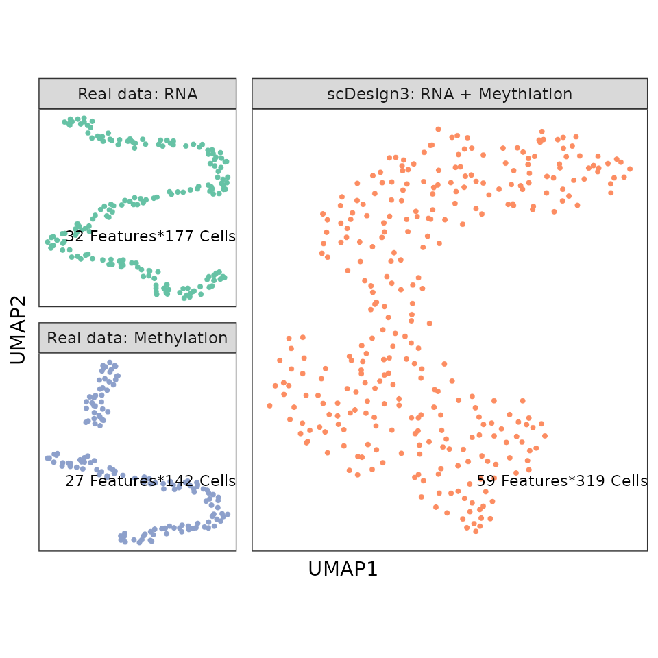
Session information
sessionInfo()
#> R version 4.3.1 (2023-06-16)
#> Platform: x86_64-pc-linux-gnu (64-bit)
#> Running under: Ubuntu 20.04.6 LTS
#>
#> Matrix products: default
#> BLAS:   /usr/lib/x86_64-linux-gnu/openblas-pthread/libblas.so.3
#> LAPACK: /usr/lib/x86_64-linux-gnu/openblas-pthread/liblapack.so.3;  LAPACK version 3.9.0
#>
#> locale:
#>  [1] LC_CTYPE=en_US.UTF-8       LC_NUMERIC=C
#>  [3] LC_TIME=en_US.UTF-8        LC_COLLATE=en_US.UTF-8
#>  [5] LC_MONETARY=en_US.UTF-8    LC_MESSAGES=en_US.UTF-8
#>  [7] LC_PAPER=en_US.UTF-8       LC_NAME=C
#>  [9] LC_ADDRESS=C               LC_TELEPHONE=C
#> [11] LC_MEASUREMENT=en_US.UTF-8 LC_IDENTIFICATION=C
#>
#> time zone: America/Los_Angeles
#> tzcode source: system (glibc)
#>
#> attached base packages:
#> [1] stats4    stats     graphics  grDevices utils     datasets  methods
#> [8] base
#>
#> other attached packages:
#>  [1] umap_0.2.10.0               ggh4x_0.2.5
#>  [3] ggplot2_3.4.2               dplyr_1.1.2
#>  [5] SingleCellExperiment_1.22.0 SummarizedExperiment_1.30.2
#>  [7] Biobase_2.60.0              GenomicRanges_1.52.0
#>  [9] GenomeInfoDb_1.36.1         IRanges_2.34.1
#> [11] S4Vectors_0.38.1            BiocGenerics_0.46.0
#> [13] MatrixGenerics_1.12.2       matrixStats_1.0.0
#> [15] scDesign3_0.99.6            BiocStyle_2.28.0
#>
#> loaded via a namespace (and not attached):
#>  [1] tidyselect_1.2.0        farver_2.1.1            vipor_0.4.5
#>  [4] bitops_1.0-7            kde1d_1.0.5             fastmap_1.1.1
#>  [7] RCurl_1.98-1.12         digest_0.6.33           lifecycle_1.0.3
#> [10] Cairo_1.6-0             survival_3.5-5          gamlss.dist_6.0-5
#> [13] magrittr_2.0.3          compiler_4.3.1          rlang_1.1.1
#> [16] sass_0.4.7              tools_4.3.1             utf8_1.2.3
#> [19] yaml_2.3.7              knitr_1.43              labeling_0.4.2
#> [22] askpass_1.1             S4Arrays_1.0.4          mclust_6.0.0
#> [25] reticulate_1.30         DelayedArray_0.26.6     RColorBrewer_1.1-3
#> [28] withr_2.5.0             purrr_1.0.1             rvinecopulib_0.6.3.1.1
#> [31] desc_1.4.2              grid_4.3.1              fansi_1.0.4
#> [34] colorspace_2.1-0        scales_1.2.1            MASS_7.3-60
#> [37] cli_3.6.1               rmarkdown_2.23          crayon_1.5.2
#> [40] ragg_1.2.5              generics_0.1.3          RSpectra_0.16-1
#> [43] ggbeeswarm_0.7.2        cachem_1.0.8            stringr_1.5.0
#> [46] zlibbioc_1.46.0         splines_4.3.1           assertthat_0.2.1
#> [49] parallel_4.3.1          ggrastr_1.0.2           BiocManager_1.30.21.1
#> [52] XVector_0.40.0          vctrs_0.6.3             Matrix_1.6-0
#> [55] jsonlite_1.8.7          bookdown_0.34           gamlss_5.4-12
#> [58] beeswarm_0.4.0          irlba_2.3.5.1           systemfonts_1.0.4
#> [61] jquerylib_0.1.4         glue_1.6.2              pkgdown_2.0.7
#> [64] rngWELL_0.10-9          stringi_1.7.12          gtable_0.3.3
#> [67] randtoolbox_2.0.4       munsell_0.5.0           tibble_3.2.1
#> [70] pillar_1.9.0            htmltools_0.5.5         openssl_2.1.0
#> [73] gamlss.data_6.0-2       GenomeInfoDbData_1.2.10 R6_2.5.1
#> [76] textshaping_0.3.6       rprojroot_2.0.3         evaluate_0.21
#> [79] lattice_0.21-8          highr_0.10              png_0.1-8
#> [82] memoise_2.0.1           bslib_0.5.0             Rcpp_1.0.11
#> [85] nlme_3.1-162            mgcv_1.9-0              xfun_0.39
#> [88] fs_1.6.3                pkgconfig_2.0.3