Perform ClusterDE on a spatial dataset (two domains)
Siqi Chen
Computer Science, Central South Universitysiqichen4477@gmail.com
Dongyuan Song
Department of Genetics & Genome Sciences, UConn HealthBioinformatics IDP, University of California, Los Angelesdongyuansong@ucla.edu
27 August 2026
Source:vignettes/ClusterDE-spatial-twodomains.Rmd
ClusterDE-spatial-twodomains.RmdDownload data
We selected adjacent layer 6 and WM of 151673 slice from the LIBD Human Dorsolateral Prefrontal Cortex (DLPFC) dataset, which is downloaded in the spatialLIBD R package. We removed the genes expressed in fewer than 20% spots to save computational time here.
data(dlpfc_twodomain, package = "ClusterDE")Visualize the real data with two domains (L6 and WM).
# Visualize the real spatial domains
domains <- data.frame(Xaxis = dlpfc_twodomain$spatial1, Yaxis = dlpfc_twodomain$spatial2, Domains = dlpfc_twodomain$cell_type)
#> Loading required namespace: SeuratObject
ggplot2::ggplot(domains, ggplot2::aes(x = Xaxis, y = Yaxis, col = Domains)) +
  ggplot2::geom_point(size = 1.0) +
  ggplot2::coord_equal() +
  ggplot2::ggtitle("Manual annotation \n (The layer6 and WM in the slice 151673)") +
  ggplot2::theme(
    plot.title = ggplot2::element_text(size = 10, hjust = 0.5),
    panel.grid = ggplot2::element_blank(),
    panel.background = ggplot2::element_rect(fill = "gray90"),
    panel.border = ggplot2::element_rect(color = "black", fill = NA, linewidth = 0.6),
    axis.title.x = ggplot2::element_blank(),
    axis.title.y = ggplot2::element_blank(),
    axis.ticks.x = ggplot2::element_blank(),
    axis.ticks.y = ggplot2::element_blank(),
    axis.text.x = ggplot2::element_blank(),
    axis.text.y = ggplot2::element_blank()
  ) +
  ggplot2::scale_color_manual(values = c("#5791cc", "#403f92"))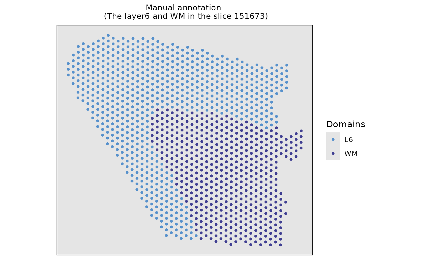
Run the BayesSpace + Seurat pipeline
First, we employed the BayesSpace for spatial clustering. Please note that ClusterDE is designed for 1 vs 1 comparison; therefore, we obtain two spatial clusters for illustration purpose.
# Construct the input of BayesSpace based on real dataset
# The input of BayesSpace is sce object
dlpfc_twodomain_sce <- SingleCellExperiment::SingleCellExperiment(
  list(counts = Seurat::GetAssayData(dlpfc_twodomain, layer = "counts"))
)
# Add colData information of SingleCellExperiment
dlpfc_twodomain_sce$row <- dlpfc_twodomain@meta.data$row
dlpfc_twodomain_sce$col <- dlpfc_twodomain@meta.data$col
dlpfc_twodomain_sce$array_row <- dlpfc_twodomain@meta.data$row
dlpfc_twodomain_sce$array_col <- dlpfc_twodomain@meta.data$col
dlpfc_twodomain_sce$spatial1 <- dlpfc_twodomain@meta.data$spatial1
dlpfc_twodomain_sce$spatial2 <- dlpfc_twodomain@meta.data$spatial2

# Log-normalize the count data
RNGkind("L'Ecuyer-CMRG")
seed <- 123
set.seed(seed)
dlpfc_twodomain_sce <- BayesSpace::spatialPreprocess(
  dlpfc_twodomain_sce,
  platform = "Visium",
  n.PCs = 7,
  log.normalize = T
)
# Clustering with BayesSpace
dlpfc_twodomain_sce <- BayesSpace::spatialCluster(
  dlpfc_twodomain_sce,
  q = 2,
  platform = "Visium",
  d = 7,
  init.method = "mclust",
  model = "t",
  gamma = 2,
  nrep = 1000,
  burn.in = 100,
  save.chain = T
)
#> Neighbors were identified for 1205 out of 1205 spots.
#> Fitting model...
#> Calculating labels using iterations 101 through 1000.
dlpfc_twodomain <- Seurat::as.Seurat(dlpfc_twodomain_sce)
#> Warning: `PackageCheck()` was deprecated in SeuratObject 5.0.0.
#> ℹ Please use `rlang::check_installed()` instead.
#> ℹ The deprecated feature was likely used in the Seurat package.
#>   Please report the issue at <https://github.com/satijalab/seurat/issues>.
#> This warning is displayed once every 8 hours.
#> Call `lifecycle::last_lifecycle_warnings()` to see where this warning was
#> generated.
#> Warning: The `slot` argument of `SetAssayData()` is deprecated as of SeuratObject 5.0.0.
#> ℹ Please use the `layer` argument instead.
#> ℹ The deprecated feature was likely used in the Seurat package.
#>   Please report the issue at <https://github.com/satijalab/seurat/issues>.
#> This warning is displayed once every 8 hours.
#> Call `lifecycle::last_lifecycle_warnings()` to see where this warning was
#> generated.
#> Warning: Keys should be one or more alphanumeric characters followed by an
#> underscore, setting key from PC to PC_
Seurat::Idents(dlpfc_twodomain) <- "spatial.cluster"
Visualize the spatial clustering results based on the real data.
# Visualize the spatial cluster
clusters <- data.frame(
  Xaxis = dlpfc_twodomain$spatial1,
  Yaxis = dlpfc_twodomain$spatial2,
  Clusters = as.character(dlpfc_twodomain$spatial.cluster)
)
ggplot2::ggplot(clusters, ggplot2::aes(x = Xaxis, y = Yaxis, col = Clusters)) +
  ggplot2::geom_point(size = 1.0) +
  ggplot2::coord_equal() +
  ggplot2::ggtitle("Real data \n (spatial clusters detected by BayesSpace)") +
  ggplot2::theme(
    plot.title = ggplot2::element_text(size = 10, hjust = 0.5),
    panel.grid = ggplot2::element_blank(),
    panel.background = ggplot2::element_rect(fill = "gray90"),
    panel.border = ggplot2::element_rect(color = "black", fill = NA, size = 0.6),
    axis.title.x = ggplot2::element_blank(),
    axis.title.y = ggplot2::element_blank(),
    axis.ticks.x = ggplot2::element_blank(),
    axis.ticks.y = ggplot2::element_blank(),
    axis.text.x = ggplot2::element_blank(),
    axis.text.y = ggplot2::element_blank()
  ) +
  ggplot2::scale_color_manual(values = c("#e87d72", "#54bcc2"))
#> Warning: The `size` argument of `element_rect()` is deprecated as of ggplot2 3.4.0.
#> ℹ Please use the `linewidth` argument instead.
#> This warning is displayed once every 8 hours.
#> Call `lifecycle::last_lifecycle_warnings()` to see where this warning was
#> generated.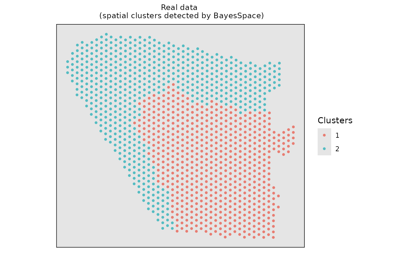
Then, we used the common DE method (Wilcoxon Rank Sum Test) to identify domain marker genes between the two spatial clusters.
original_deg <- Seurat::FindMarkers(
  object = dlpfc_twodomain,
  ident.1 = 2,
  ident.2 = 1,
  test.use = "wilcox",
  logfc.threshold = 0,
  min.pct = 0,
  min.cells.feature = 1,
  min.cells.group = 1
)
#> Warning: The `slot` argument of `GetAssayData()` is deprecated as of SeuratObject 5.0.0.
#> ℹ Please use the `layer` argument instead.
#> ℹ The deprecated feature was likely used in the Seurat package.
#>   Please report the issue at <https://github.com/satijalab/seurat/issues>.
#> This warning is displayed once every 8 hours.
#> Call `lifecycle::last_lifecycle_warnings()` to see where this warning was
#> generated.
original_pval <- original_deg$p_val_adj
names(original_pval) <- rownames(original_deg)
print(paste0("Seurat found ", sum(original_deg$p_val_adj < 0.05), " DEG"))
#> [1] "Seurat found 1234 DEG"
Find DEGs using ClusterDE
We use spatial coordinates as covariates to generate synthetic null data, then apply the same BayesSpace clustering method as target data. This may take a few minutes to run.
set.seed(seed)
null_data <- ClusterDE::constructNull(
  dlpfc_twodomain,
  data_type = "spatial",
  formula = "s(spatial1, spatial2, bs = 'gp', k = 4)",
  other_covariates = c("spatial1", "spatial2")
)
#> Registered S3 method overwritten by 'gamlss':
#>   method   from
#>   print.ri bit
#> Registered S3 method overwritten by 'scDesign3':
#>   method         from
#>   predict.gamlss gamlss
#> Input Data Construction Start
#> Input Data Construction End
#> Start Marginal Fitting
#> Marginal Fitting End
#> Start Copula Fitting
#> Convert Residuals to Multivariate Gaussian
#> Converting End
#> Copula group 1 starts
#> Copula Fitting End
#> Start Parameter Extraction
#> Parameter
#> Extraction End
#> Start Generate New Data
#> Use Copula to sample a multivariate quantile matrix
#> Sample Copula group 1 starts
#> New Data Generating End
null_obj_sce <- SingleCellExperiment::SingleCellExperiment(list(counts = null_data))
null_obj_sce$row <- dlpfc_twodomain@meta.data$row
null_obj_sce$col <- dlpfc_twodomain@meta.data$col
null_obj_sce$array_row <- dlpfc_twodomain@meta.data$row
null_obj_sce$array_col <- dlpfc_twodomain@meta.data$col
null_obj_sce$spatial1 <- dlpfc_twodomain@meta.data$spatial1
null_obj_sce$spatial2 <- dlpfc_twodomain@meta.data$spatial2
null_obj_sce <- BayesSpace::spatialPreprocess(
  null_obj_sce,
  platform = "Visium",
  n.PCs = 7,
  log.normalize = T
)
null_obj_sce <- BayesSpace::spatialCluster(
  null_obj_sce,
  q = 2,
  platform = "Visium",
  d = 7,
  init.method = "mclust",
  model = "t",
  gamma = 2,
  nrep = 1000,
  burn.in = 100,
  save.chain = T
)
#> Neighbors were identified for 1205 out of 1205 spots.
#> Fitting model...
#> Calculating labels using iterations 101 through 1000.
null_obj <- Seurat::as.Seurat(null_obj_sce)
#> Warning: Keys should be one or more alphanumeric characters followed by an
#> underscore, setting key from PC to PC_
Seurat::Idents(null_obj) <- "spatial.cluster"
Compare gene p-values from target and synthetic data to calculate ClusterDE FDR controlled DEG.
null_deg <- Seurat::FindMarkers(
  object = null_obj,
  ident.1 = 1,
  ident.2 = 2,
  test.use = "wilcox",
  logfc.threshold = 0,
  min.pct = 0,
  min.cells.feature = 1,
  min.cells.group = 1
)
null_pval <- null_deg$p_val_adj
names(null_pval) <- rownames(null_deg)

deg <- ClusterDE::callDE(original_pval, null_pval)
print(paste0("ClusterDE found ", sum(deg$record >= 0.5), " DEG"))
#> [1] "ClusterDE found 929 DEG"
Session information
sessionInfo()
#> R version 4.5.1 (2025-06-13)
#> Platform: x86_64-pc-linux-gnu
#> Running under: Ubuntu 24.04.4 LTS
#>
#> Matrix products: default
#> BLAS/LAPACK: FlexiBLAS OPENBLAS;  LAPACK version 3.12.0
#>
#> Random number generation:
#>  RNG:     L'Ecuyer-CMRG
#>  Normal:  Inversion
#>  Sample:  Rejection
#>
#> locale:
#>  [1] LC_CTYPE=C.UTF-8       LC_NUMERIC=C           LC_TIME=C.UTF-8
#>  [4] LC_COLLATE=C.UTF-8     LC_MONETARY=C.UTF-8    LC_MESSAGES=C.UTF-8
#>  [7] LC_PAPER=C.UTF-8       LC_NAME=C              LC_ADDRESS=C
#> [10] LC_TELEPHONE=C         LC_MEASUREMENT=C.UTF-8 LC_IDENTIFICATION=C
#>
#> time zone: America/Los_Angeles
#> tzcode source: system (glibc)
#>
#> attached base packages:
#> [1] stats     graphics  grDevices utils     datasets  methods   base
#>
#> other attached packages:
#> [1] BiocStyle_2.36.0
#>
#> loaded via a namespace (and not attached):
#>   [1] fs_1.6.6                    matrixStats_1.5.0
#>   [3] spatstat.sparse_3.1-0       bitops_1.0-9
#>   [5] httr_1.4.7                  RColorBrewer_1.1-3
#>   [7] backports_1.5.0             tools_4.5.1
#>   [9] sctransform_0.4.2           R6_2.6.1
#>  [11] DirichletReg_0.7-2          mgcv_1.9-3
#>  [13] lazyeval_0.2.2              uwot_0.2.3
#>  [15] rhdf5filters_1.20.0         withr_3.0.2
#>  [17] sp_2.2-0                    ClusterDE_0.99.4
#>  [19] gridExtra_2.3               progressr_0.15.1
#>  [21] cli_3.6.5                   Biobase_2.68.0
#>  [23] textshaping_1.0.1           spatstat.explore_3.4-3
#>  [25] fastDummies_1.7.5           microbenchmark_1.5.0
#>  [27] sandwich_3.1-1              labeling_0.4.3
#>  [29] sass_0.4.10                 Seurat_5.3.0
#>  [31] mvtnorm_1.3-3               arrow_20.0.0.2
#>  [33] spatstat.data_3.1-6         gamlss_5.4-22
#>  [35] ggridges_0.5.6              pbapply_1.7-2
#>  [37] pkgdown_2.0.9               systemfonts_1.2.3
#>  [39] dichromat_2.0-0.1           scater_1.36.0
#>  [41] parallelly_1.45.0           limma_3.64.1
#>  [43] RSQLite_2.4.1               gamlss.data_6.0-6
#>  [45] generics_0.1.4              ica_1.0-3
#>  [47] spatstat.random_3.4-1       dplyr_1.1.4
#>  [49] Matrix_1.7-5                ggbeeswarm_0.7.2
#>  [51] S4Vectors_0.46.0            abind_1.4-8
#>  [53] lifecycle_1.0.4             yaml_2.3.10
#>  [55] edgeR_4.6.2                 SummarizedExperiment_1.38.1
#>  [57] rhdf5_2.52.1                SparseArray_1.8.0
#>  [59] BiocFileCache_2.16.0        Rtsne_0.17
#>  [61] grid_4.5.1                  blob_1.2.4
#>  [63] promises_1.3.3              dqrng_0.4.1
#>  [65] crayon_1.5.3                miniUI_0.1.2
#>  [67] lattice_0.22-9              beachmat_2.24.0
#>  [69] cowplot_1.1.3               pillar_1.10.2
#>  [71] knitr_1.50                  metapod_1.16.0
#>  [73] GenomicRanges_1.60.0        rjson_0.2.23
#>  [75] xgboost_3.2.1.1             future.apply_1.20.0
#>  [77] codetools_0.2-20            glue_1.8.0
#>  [79] spatstat.univar_3.1-3       data.table_1.17.4
#>  [81] vctrs_0.6.5                 png_0.1-8
#>  [83] spam_2.11-1                 gtable_0.3.6
#>  [85] assertthat_0.2.1            cachem_1.1.0
#>  [87] xfun_0.52                   S4Arrays_1.8.1
#>  [89] mime_0.13                   coda_0.19-4.1
#>  [91] survival_3.8-3              SingleCellExperiment_1.30.1
#>  [93] maxLik_1.5-2.1              statmod_1.5.0
#>  [95] bluster_1.18.0              BayesSpace_1.21.2
#>  [97] fitdistrplus_1.2-2          ROCR_1.0-11
#>  [99] bettermc_1.2.2.9000         nlme_3.1-168
#> [101] bit64_4.6.0-1               filelock_1.0.3
#> [103] RcppAnnoy_0.0.22            GenomeInfoDb_1.44.0
#> [105] bslib_0.9.0                 irlba_2.3.5.1
#> [107] vipor_0.4.7                 KernSmooth_2.23-26
#> [109] BiocGenerics_0.54.0         DBI_1.2.3
#> [111] tidyselect_1.2.1            bit_4.6.0
#> [113] compiler_4.5.1              curl_6.3.0
#> [115] BiocNeighbors_2.2.0         desc_1.4.3
#> [117] DelayedArray_0.34.1         plotly_4.10.4
#> [119] bookdown_0.43               checkmate_2.3.2
#> [121] scales_1.4.0                lmtest_0.9-40
#> [123] stringr_1.5.1               digest_0.6.37
#> [125] goftest_1.2-3               presto_1.0.0
#> [127] spatstat.utils_3.1-4        rmarkdown_2.29
#> [129] scDesign3_1.7.6             XVector_0.48.0
#> [131] htmltools_0.5.8.1           pkgconfig_2.0.3
#> [133] MatrixGenerics_1.20.0       dbplyr_2.5.0
#> [135] fastmap_1.2.0               rlang_1.1.6
#> [137] htmlwidgets_1.6.4           UCSC.utils_1.4.0
#> [139] shiny_1.10.0                farver_2.1.2
#> [141] jquerylib_0.1.4             zoo_1.8-14
#> [143] jsonlite_2.0.0              BiocParallel_1.42.1
#> [145] mclust_6.1.1                BiocSingular_1.24.0
#> [147] RCurl_1.98-1.17             magrittr_2.0.3
#> [149] Formula_1.2-5               scuttle_1.18.0
#> [151] GenomeInfoDbData_1.2.14     dotCall64_1.2
#> [153] patchwork_1.3.0             Rhdf5lib_1.30.0
#> [155] Rcpp_1.0.14                 viridis_0.6.5
#> [157] reticulate_1.42.0           stringi_1.8.7
#> [159] MASS_7.3-65                 gamlss.dist_6.1-1
#> [161] plyr_1.8.9                  parallel_4.5.1
#> [163] listenv_0.9.1               ggrepel_0.9.6
#> [165] deldir_2.0-4                splines_4.5.1
#> [167] tensor_1.5                  locfit_1.5-9.12
#> [169] igraph_2.1.4                spatstat.geom_3.4-1
#> [171] RcppHNSW_0.6.0              reshape2_1.4.4
#> [173] stats4_4.5.1                ScaledMatrix_1.16.0
#> [175] evaluate_1.0.3              SeuratObject_5.1.0
#> [177] scran_1.36.0                BiocManager_1.30.27
#> [179] httpuv_1.6.16               miscTools_0.6-28
#> [181] RANN_2.6.2                  tidyr_1.3.1
#> [183] purrr_1.0.4                 polyclip_1.10-7
#> [185] future_1.58.0               scattermore_1.2
#> [187] ggplot2_3.5.2               rsvd_1.0.5
#> [189] xtable_1.8-4                RSpectra_0.16-2
#> [191] later_1.4.2                 viridisLite_0.4.2
#> [193] ragg_1.4.0                  tibble_3.3.0
#> [195] memoise_2.0.1               beeswarm_0.4.0
#> [197] IRanges_2.42.0              cluster_2.1.8.1
#> [199] globals_0.18.0